Plot of diffraction patterns

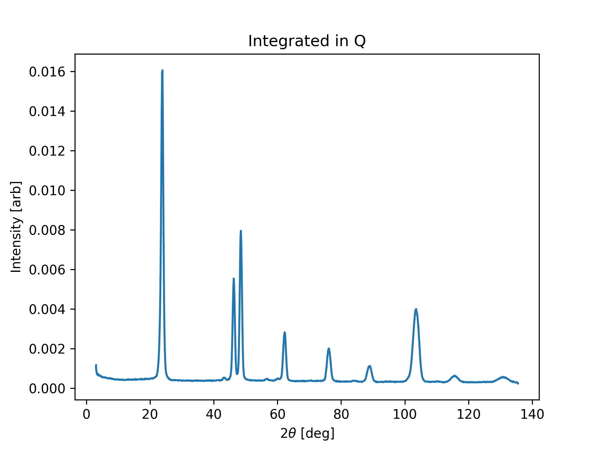
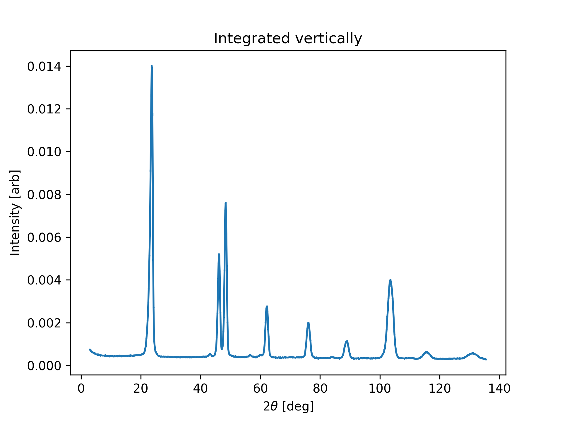
When a powder sample has been measured at DMC it is saved in hdf files. Several DataFiles can be combined into a common DataSet and plotted. The follwing code takes a DatsSet, here consisting of several DataFiles, and plot the dataSet. Two different settings for the binning method is used correctedTwoTheta equal to True and False. When False a naive summation across the 2D detector is performed where the out-of-plane component is not taken into account. That is, summation is performed vertically on the detector. For powder patterns around 90^o, this is only a very minor error, but for scattering close to the direct beam a significant error is introduced. Instead, utilizing correctedTwoTheta = True is the correct way. The scattering 3D vector is calculated for each individual pixel on the 2D detector and it’s length is calculated.

from DMCpy import DataSet,DataFile, _tools
import matplotlib.pyplot as plt

# To plot powder data we give the file number, or list of filenumbers as a string and the folder of the raw data
scanNumbers = '1285-1290'
folder = 'data'
year = 2022

# a list of dataFiles are generated with loadDataFile running over all the dataFiles generated from _tools.fileListGenerator and twoThetaOffset acts on the dataFile
dataFiles = [DataFile.loadDataFile(dFP) for dFP in _tools.fileListGenerator(scanNumbers,folder,year=year)]

# We then create a data set based on the data files
ds = DataSet.DataSet(dataFiles)

for df in ds:
   df.generateMask(lambda x: DataFile.maskFunction(x,maxAngle=180.0),replace=True)
ds._getData()

# We can also give the step size for the integration. Default is 0.125
dTheta = 0.125

# Generate a diffraction pattern where the 2D detector is integrated in Q-space
ax,bins,Int,Int_err,monitor = ds.plotTwoTheta(dTheta=dTheta)
ax.set_title('Integrated in Q')
fig = ax.get_figure()
fig.savefig('figure0.png',format='png'),r'docs/Tutorials/Powder/TwoThetaPowderQ.png'),format='png',dpi=300)

# Generate a diffraction pattern where the 2D detector is integrated vertically
# Note that when correctedTwoTheta, the x-axis is negaive and must be inverted
ax2,bins2,Int2,Int_err2,monitor2 = ds.plotTwoTheta(correctedTwoTheta=False,dTheta=dTheta)
ax2.set_title('Integrated vertically')
fig2 = ax2.get_figure()
fig2.savefig('figure1.png',format='png'),r'docs/Tutorials/Powder/TwoThetaPowderVertical.png'),format='png',dpi=300)

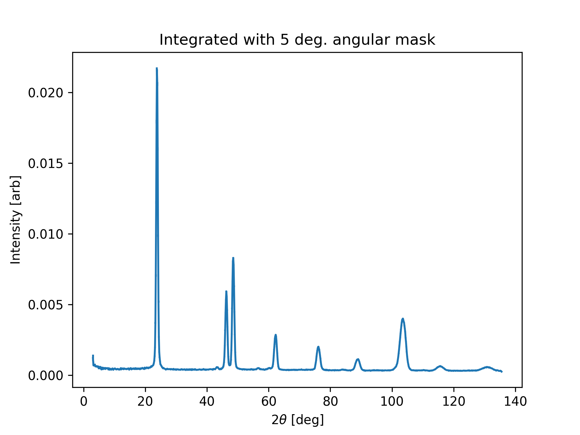
# Generate a diffraction pattern where the 2D detector is integrated in Q-space with and 5 deg. angular mask
for df in ds:
   df.generateMask(lambda x: DataFile.maskFunction(x,maxAngle=5.0),replace=True)
# for powder integration we need to use _getData() to apply the mask
ds._getData()

ax3,bins3,Int3,Int_err3,monitor3 = ds.plotTwoTheta(dTheta=dTheta)
ax3.set_title('Integrated with 5 deg. angular mask')
fig3 = ax3.get_figure()
fig3.savefig('figure2.png',format='png'),r'docs/Tutorials/Powder/TwoThetaPowderMask.png'),format='png',dpi=300)

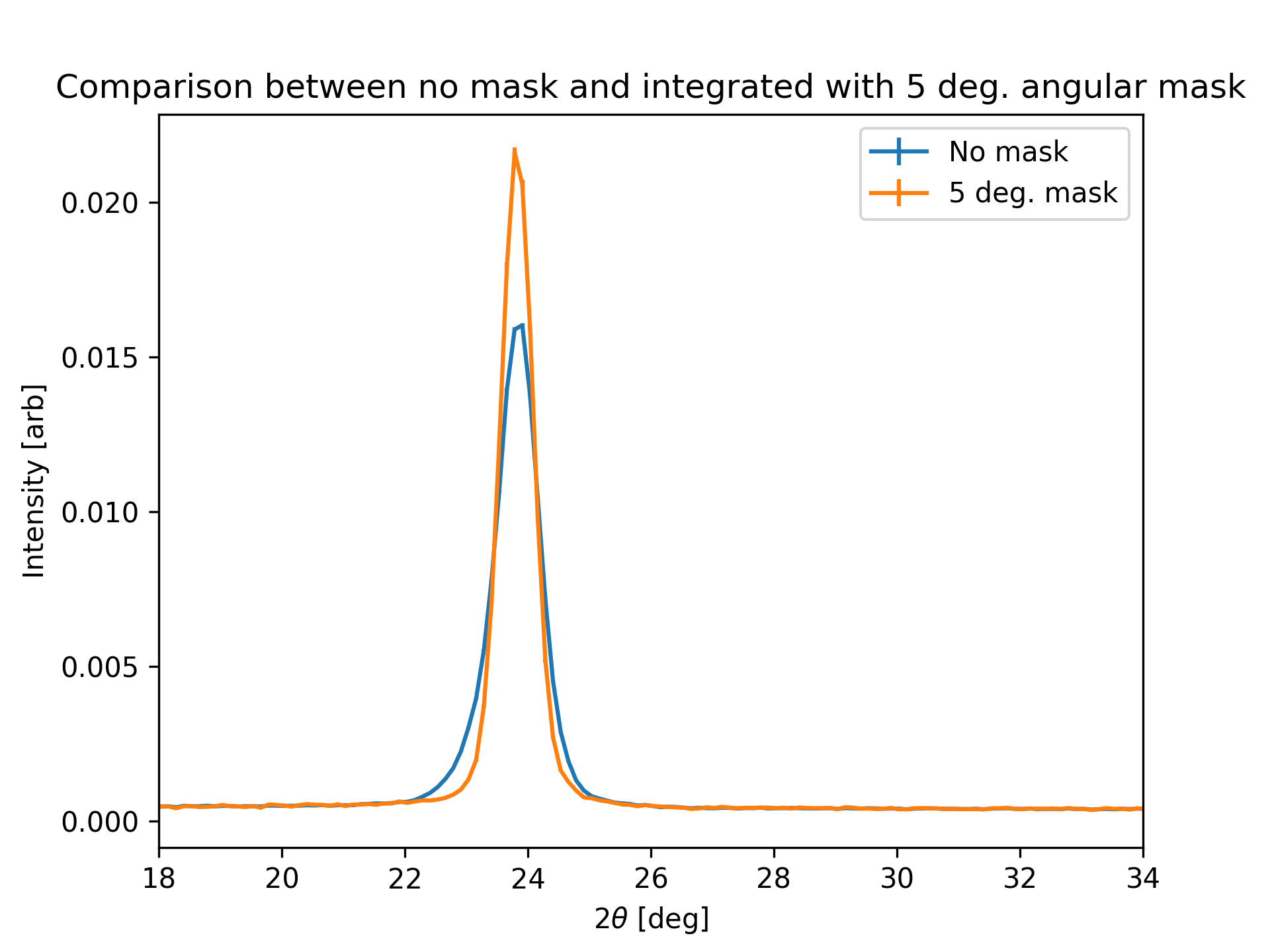
# plot integration with and without mask together
fig4,ax4 = plt.subplots()
ax4.set_title('Comparison between no mask and integrated with 5 deg. angular mask')
ax4.set_xlabel(r'$2\theta$ [deg]')
ax4.set_ylabel(r'Intensity [arb]')
# bins are the limits and we need to take the average to get corrct xbins
plt.errorbar(0.5*(bins[1:]+bins[:-1]),Int,yerr=Int_err,label='No mask')
plt.errorbar(0.5*(bins3[1:]+bins3[:-1]),Int3,yerr=Int_err3,label='5 deg. mask')
plt.xlim(18,34)
ax4.legend()
fig4.savefig('figure3.png',format='png'),r'docs/Tutorials/Powder/TwoThetaPowderCombined.png'),format='png',dpi=300)

# plot integration with Q integration and vertical integration
fig5,ax5 = plt.subplots()
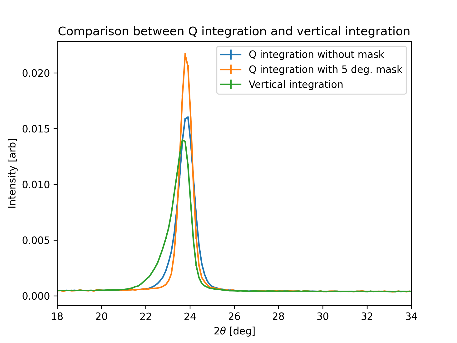
ax5.set_title('Comparison between Q integration and vertical integration')
ax5.set_xlabel(r'$2\theta$ [deg]')
ax5.set_ylabel(r'Intensity [arb]')
plt.errorbar(0.5*(bins[1:]+bins[:-1]),Int,yerr=Int_err,label='Q integration without mask')
plt.errorbar(0.5*(bins3[1:]+bins3[:-1]),Int3,yerr=Int_err3,label='Q integration with 5 deg. mask')
plt.errorbar(0.5*(bins2[1:]+bins2[:-1]),Int2,yerr=Int_err2,label='Vertical integration')
plt.xlim(18,34)
ax5.legend()
fig5.savefig('figure4.png',format='png'),r'docs/Tutorials/Powder/TwoThetaPowderCombined2.png'),format='png',dpi=300)

Running the above code generates the following, similar looking, diffractograms utilizing the corrected and uncorrected twoTheta positions respectively. We highlight the reduced noice and the slightly sharper peaks in the corrected image.The down-up glitches of the diffraction pattern is from the interface between the detector sections. Integration with different masks and comparisons are also displayed.