Cut2D hk0

After inspecting the scattering plane, we want to perform cuts along certain directions. In this tutorial, we demonstrate the cut2D function. Cuts can be made given by hkl or Qx, Qy, Qz, by using rlu=True/False. The width of the cut orthogonal to the plane can be adjusted by the keywords width. The grid the cut is projected on is given by the xBins and yBins keywords or dQx and dQy. The binning is allways given in Q-space, also when you do a cut in HKL-space. The unit of width and binning is AA-1.

import matplotlib.pyplot as plt
from DMCpy import DataSet,DataFile,_tools
import numpy as np

# Give file number and folder the file is stored in.
scanNumbers = '12153-12154'
folder = 'data/SC'
year = 2022

filePath = _tools.fileListGenerator(scanNumbers,folder,year=year)

unitCell = np.array([ 7.218, 7.218, 18.183, 90.0, 90.0, 120.0])

# # # load dataFiles
dataFiles = [DataFile.loadDataFile(dFP,unitCell = unitCell) for dFP in filePath]

# load data files and make data set
ds = DataSet.DataSet(dataFiles)

# Define Q coordinates and HKL for the coordinates.
q1 = [-0.447,-0.914,-0.003]
q2 = [-1.02,-0.067,-0.02]
HKL1 = [1,0,0]
HKL2 = [0,1,0]

# this function uses two coordinates in Q space and align them to corrdinates in HKL space
ds.alignToRefs(q1=q1,q2=q2,HKL1=HKL1,HKL2=HKL2)

# define 2D cut width orthogonal to cut plane
width = 0.5

# these points define the plane that will be cut
points = np.array([[0.0,0.0,0.0],
     [1.0,0.0,0.0],
     [0.0,1.0,0.0]])

kwargs = {
   'dQx' : 0.01,
   'dQy' : 0.01,
   'steps' : 151,
   'rlu' : True,
   'rmcFile' : True,
   'colorbar' : True,
   }

ax,returndata,bins = ds.plotQPlane(points=points,width=width,**kwargs)

ax.set_clim(0,0.0001)

planeFigName = 'docs/Tutorials/2Dcut_hk0'
plt.savefig('figure0.png',format='png')

# save csv and txt file with data
if False:
   kwargs = {
   'rmcFileName' : planeFigName+'.txt'
   }

   ax.to_csv(planeFigName+'.csv',**kwargs)


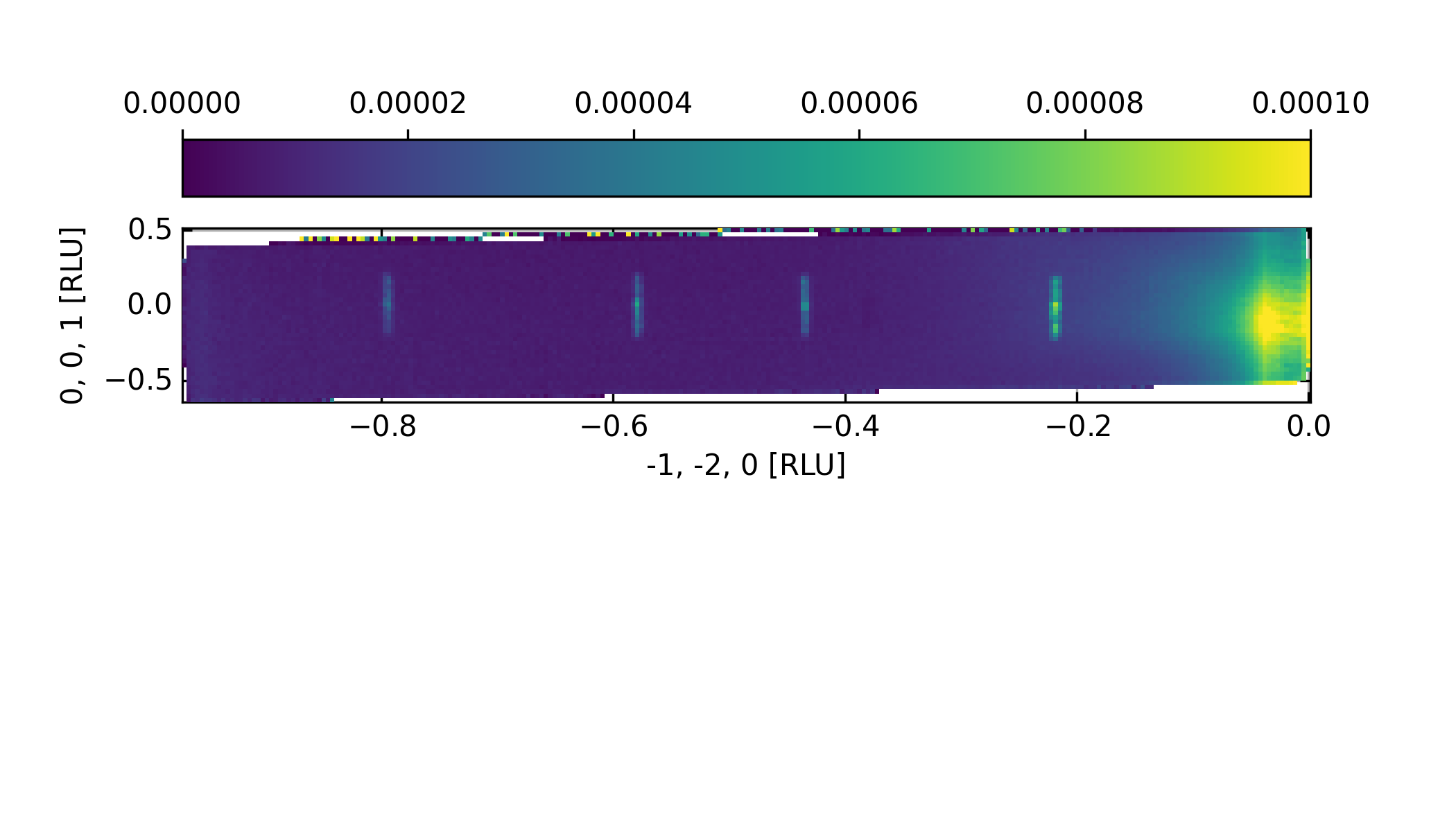
# cut 2D plane orhtogonal to scattering plane
width = 0.5

points = np.array([[0.0,0.0,0.0],
     [-1.0,-2.0,0.0],
     [0.0,0.0,1.0]])

kwargs = {
   'dQx' : 0.01,
   'dQy' : 0.01,
   'steps' : 151,
   'rlu' : True,
   'rmcFile' : True,
   'colorbar' : True,
   }

ax,returndata,bins = ds.plotQPlane(points=points,width=width,**kwargs)

ax.set_clim(0,0.0001)
ax.set_xticks_number(7)
ax.set_yticks_number(3)

ax.colorbar.set_label('')
ax.colorbar.remove()
plt.gcf().colorbar(ax.colorbar.mappable,ax=ax,orientation='horizontal', location='top')

planeFigName = 'docs/Tutorials/2Dcut_hk0_side'
plt.savefig('figure1.png',format='png')

if False:
   kwargs = {
   'rmcFileName' : planeFigName+'.txt'
   }

   ax.to_csv(planeFigName+'.csv',**kwargs)

The above code takes the data from the A3 scan files dmc2022n012153-dmc2022n012154, align and plot the scattering plane.

Figure of the 2D plane in RLU.

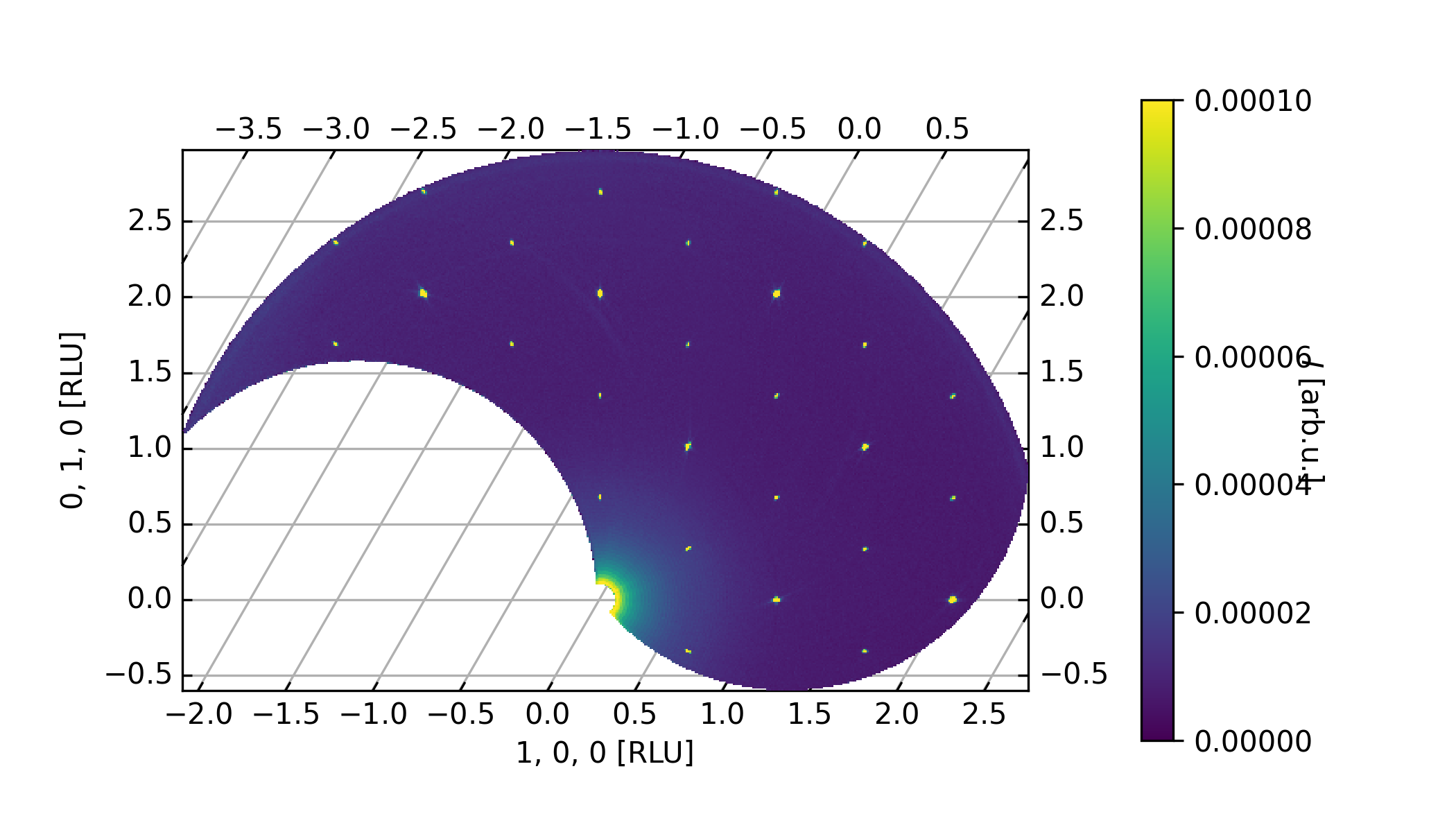
Figure of the 2D plane in RLU.